
* 티스토리에서 마크다운 적용이 안돼서 깨지는 부분이 많습니다.
* 깨지지 않은 파일로 자세히 보기 원하시는 분들은 아래 링크 참고해주세요!
파이썬 머신러닝 완벽 가이드 - 3. Scikit-Learn
Classifier 분류: DecisionTreeClassifier, RandomForestClassifier, GradientBoostingClassifier, GaussianNB, SVCRegressor 회귀: LinearRegression, Ridge, Lasso
velog.io

Scikit-Learn 사이킷런
1. Estimator
1. Classifier 분류
: DecisionTreeClassifier, RandomForestClassifier, GradientBoostingClassifier, GaussianNB, SVC2. Regressor 회귀
: LinearRegression, Ridge, Lasso, RandomForestRegressor, GradientBoostingRegressor3. 비지도학습/피처추출(전처리) 에서의 fit(), transform()
: fit()이 학습이 아니라, 입력 데이터 형태에 맞춰 데이터를 변환하기 위한 사전 구조를 맞추는 작업
: transform()은 fit으로 변환된 사전 구조를 가지고 차원변환/클러스터링/피처추출 등을 하는 작업
2. Module
- sklearn.model_selection 의
train_test_split(features, labels, test_size)
교차 검증: 데이터 편중을 막기 위해 별도의 여러 세트로 구성된 학습 데이터 세트와 검증 데이터 세트에서 학습, 평가를 수행하는 것
- KFold : K개의 데이터 폴드 세트를 만들어서, K번만큼 각 폴드 세트에 학습과 검증 평가를 반복적으로 수행하는 방법
- KFold(n_splits = 폴드 개수)
- split( ): 학습용/검증용 데이터로 분할할 수 있는, 각각의 인덱스를 반환
- 객체 생성
- 인덱스 얻기
- 인덱스 활용해 데이터 추출
- 학습
- 예측
- 정확도 측정
- 평균 정확도
- Kfold 사용 예시 코드
        kfold = KFold(n_splits=5)
        cv_accuracy = []

        n_iter = 0

        # KFold객체의 split( ) 호출하면 폴드 별 학습용, 검증용 테스트의 로우 인덱스를 array로 반환
        for train_index, test_index  in kfold.split(features):
            # kfold.split( )으로 반환된 인덱스를 이용하여 학습용, 검증용 테스트 데이터 추출
            X_train, X_test = features[train_index], features[test_index]
            y_train, y_test = label[train_index], label[test_index]
            #학습 및 예측
            dt_clf.fit(X_train , y_train)
            pred = dt_clf.predict(X_test)
            n_iter += 1
            # 반복 시 마다 정확도 측정
            accuracy = np.round(accuracy_score(y_test,pred), 4)
            train_size = X_train.shape[0]
            test_size = X_test.shape[0]
            print('\n#{0} 교차 검증 정확도 :{1}, 학습 데이터 크기: {2}, 검증 데이터 크기: {3}'
                  .format(n_iter, accuracy, train_size, test_size))
            print('#{0} 검증 세트 인덱스:{1}'.format(n_iter,test_index))
            cv_accuracy.append(accuracy)

        # 개별 iteration별 정확도를 합하여 평균 정확도 계산
        print('\n## 평균 검증 정확도:', np.mean(cv_accuracy))


    - Kfold 사용 예시 코드 결과

        > #1 교차 검증 정확도 :1.0, 학습 데이터 크기: 120, 검증 데이터 크기: 30
        #1 검증 세트 인덱스:[ 0  1  2  3  4  5  6  7  8  9 10 11 12 13 14 15 16 17 18 19 20 21 22 23 24 25 26 27 28 29]

        #2 교차 검증 정확도 :0.9667, 학습 데이터 크기: 120, 검증 데이터 크기: 30
        #2 검증 세트 인덱스:[30 31 32 33 34 35 36 37 38 39 40 41 42 43 44 45 46 47 48 49 50 51 52 53 54 55 56 57 58 59]

        #3 교차 검증 정확도 :0.8667, 학습 데이터 크기: 120, 검증 데이터 크기: 30
        #3 검증 세트 인덱스:[60 61 62 63 64 65 66 67 68 69 70 71 72 73 74 75 76 77 78 79 80 81 82 83 84 85 86 87 88 89]

        #4 교차 검증 정확도 :0.9333, 학습 데이터 크기: 120, 검증 데이터 크기: 30
        #4 검증 세트 인덱스:[ 90  91  92  93  94  95  96  97  98  99 100 101 102 103 104 105 106 107 108 109 110 111 112 113 114 115 116 117 118 119]

        #5 교차 검증 정확도 :0.7333, 학습 데이터 크기: 120, 검증 데이터 크기: 30
        #5 검증 세트 인덱스:[120 121 122 123 124 125 126 127 128 129 130 131 132 133 134 135 136 137 138 139 140 141 142 143 144 145 146 147 148 149]

## 평균 검증 정확도: 0.9- Stratified KFold : 레이블 데이터 분포도에 따라 학습/검증 데이터를 나눔
⇒ 회귀에서는 연속형 데이터라 (not 이산형) Stratify가 의미가 없음- split(features, labels) : split에 피처, 레이블 데이터 모두를 입력해야 한다.
- Stratified Kfold 사용 예시 코드
iris = load_iris()
features = iris.data
label = iris.target

dt_clf = DecisionTreeClassifier(random_state=156)

skfold = StratifiedKFold(n_splits=3)
n_iter=0
cv_accuracy=[]

# StratifiedKFold의 split( ) 호출시 반드시 레이블 데이터 셋도 추가 입력 필요
for train_index, test_index  in skfold.split(features, label):
    # split( )으로 반환된 인덱스를 이용하여 학습용, 검증용 테스트 데이터 추출
    X_train, X_test = features[train_index], features[test_index]
    y_train, y_test = label[train_index], label[test_index]
    #학습 및 예측
    dt_clf.fit(X_train , y_train)
    pred = dt_clf.predict(X_test)

    # 반복 시 마다 정확도 측정
    n_iter += 1
    accuracy = np.round(accuracy_score(y_test,pred), 4)
    train_size = X_train.shape[0]
    test_size = X_test.shape[0]
    print('\n#{0} 교차 검증 정확도 :{1}, 학습 데이터 크기: {2}, 검증 데이터 크기: {3}'
          .format(n_iter, accuracy, train_size, test_size))
    print('#{0} 검증 세트 인덱스:{1}'.format(n_iter,test_index))
    cv_accuracy.append(accuracy)

# 교차 검증별 정확도 및 평균 정확도 계산
print('\n## 교차 검증별 정확도:', np.round(cv_accuracy, 4))
print('## 평균 검증 정확도:', np.mean(cv_accuracy))


### Stratified Kfold 사용 예시 코드 결과

#1 교차 검증 정확도 :0.98, 학습 데이터 크기: 100, 검증 데이터 크기: 50
#1 검증 세트 인덱스:[  0   1   2   3   4   5   6   7   8   9  10  11  12  13  14  15  16  50
51  52  53  54  55  56  57  58  59  60  61  62  63  64  65  66 100 101
102 103 104 105 106 107 108 109 110 111 112 113 114 115]

#2 교차 검증 정확도 :0.94, 학습 데이터 크기: 100, 검증 데이터 크기: 50
#2 검증 세트 인덱스:[ 17  18  19  20  21  22  23  24  25  26  27  28  29  30  31  32  33  67
68  69  70  71  72  73  74  75  76  77  78  79  80  81  82 116 117 118
119 120 121 122 123 124 125 126 127 128 129 130 131 132]

#3 교차 검증 정확도 :0.98, 학습 데이터 크기: 100, 검증 데이터 크기: 50
#3 검증 세트 인덱스:[ 34  35  36  37  38  39  40  41  42  43  44  45  46  47  48  49  83  84
85  86  87  88  89  90  91  92  93  94  95  96  97  98  99 133 134 135
136 137 138 139 140 141 142 143 144 145 146 147 148 149]

## 교차 검증별 정확도: [0.98 0.94 0.98]
## 평균 검증 정확도: 0.9666666666666667
- cross_val_score(estimator, feartures, labels, scoring=단일_예측성능_평가지표, cv=교차검증_폴드수) : 교차 검증 편하게 used Stratified KFold
- cross_validation(estimator, feartures, labels, scoring=[복수_예측성능_평가지표], cv=교차검증_폴드수) : 여러 개의 평가지표를 반환
GridSearchCV(estimator, param_grid=파라미터 값 딕셔너리, scoring=평가지표, cv=분할되는 학습/테스트 세트 개수, refit=True): 교차 검증 + 최적 파라미터 튜닝을 한 번에refit: 최적 하이퍼 파라미터로 재학습한다. ⇒ default가 True임- cf) 평가지표들
  from sklearn.metrics import SCORERS
  SCORERS.keys()
- GridSearchCV 사용 예시 코드
dtree = DecisionTreeClassifier()

# parameter 들을 dictionary 형태로 설정
parameters = {'max_depth':[1,2,3], 'min_samples_split':[2,3]}

grid_dtree = GridSearchCV(dtree, param_grid=parameters, scoring='accuracy' , cv=3, refit=True)
# 이렇게 multi-metric 줄 수도 있음 => refit을 어떤 metric으로 할지 설정해줘야함
grid_dtree = GridSearchCV(dtree, param_grid=parameters, scoring=['accuracy', 'r2'] , cv=3, refit='accuracy')

# 붓꽃 Train 데이터로 param_grid의 하이퍼 파라미터들을 순차적으로 학습/평가 .
grid_dtree.fit(X_train, y_train)

# GridSearchCV 결과 추출하여 DataFrame으로 변환
scores_df = pd.DataFrame(grid_dtree.cv_results_)
scores_df[['params', 'mean_test_score', 'rank_test_score', \
           'split0_test_score', 'split1_test_score', 'split2_test_score']]

print('GridSearchCV 최적 파라미터:', grid_dtree.best_params_)
print('GridSearchCV 최고 정확도: {0:.4f}'.format(grid_dtree.best_score_))


# GridSearchCV의 refit으로 이미 학습이 된 estimator 반환
estimator = grid_dtree.best_estimator_

# GridSearchCV의 best_estimator_는 이미 최적 하이퍼 파라미터로 학습이 됨
pred = estimator.predict(X_test)
print('테스트 데이터 세트 정확도: {0:.4f}'.format(accuracy_score(y_test,pred)))
3. 데이터 전처리
: 사이킷런 머신러닝에서 문자열과 NaN은, 입력값이 될 수 없다 → 숫자형이어야만 함 → 인코딩이 필수적
3.1.레이블 인코딩 (Label encoding) : 카테고리 피처를 코드형 숫자값으로 변환
LabelEncoder(): 객체생성 →fit_transform()←inverse_transform(): 디코딩- 레이블 인코딩 과정
from sklearn.preprocessing import LabelEncoder

items=['TV','냉장고','전자렌지','컴퓨터','선풍기','선풍기','믹서','믹서']

# LabelEncoder를 객체로 생성한 후 , fit( ) 과 transform( ) 으로 label 인코딩 수행.
encoder = LabelEncoder()
encoder.fit(items)
labels = encoder.transform(items)

print('인코딩 변환값:',labels)
print('인코딩 클래스:',encoder.classes_)
print('디코딩 원본 값:',encoder.inverse_transform([4, 5, 2, 0, 1, 1, 3, 3]))

> 인코딩 변환값: [0 1 4 5 3 3 2 2]
> 인코딩 클래스: ['TV' '냉장고' '믹서' '선풍기' '전자렌지' '컴퓨터']
> 디코딩 원본 값: ['전자렌지' '컴퓨터' '믹서' 'TV' '냉장고' '냉장고' '선풍기' '선풍기']inverse_transform(): 디코딩- Label Encoding은 숫자의 크기에 따라 순서나, 중요도 등의 가중치로 반영될 수 있으므로, 선형회귀와 같은 ML 알고리즘에는 적용되지 않아야 함
- 트리 계열의 ML 알고리즘은 숫자의 이러한 특성을 반영하지 않으므로, 레이블 인코딩도 별 문제가 없음
3.2. 원-핫 인코딩 (One-Hot encoding) : 피처 값의 유형에 따라 고유 값에 해당 칼럼만 1 표시 / 나머지는 0
- 원-핫 인코더로 변환하기 전, 모든 문자열 값이 숫자형 값으로 변환 돼야 한다 (used by
LabelEncoder())- == 원-핫 인코더의 input으로 숫자형이 와야한다
- 입력값으로 2차원 데이터가 필요하다는 것 (used by
reshape(-1, 1)) LabelEncoder(): 객체생성 →fit_transform()→labels.reshape(-1, 1)→OneHotEncoder()→fit_transform()←inverse_transform(): 디코딩- 원-핫 인코딩 과정
items=['TV','냉장고','전자렌지','컴퓨터','선풍기','선풍기','믹서','믹서']

# 먼저 숫자값으로 변환을 위해 LabelEncoder로 변환합니다.
encoder = LabelEncoder()
encoder.fit(items)
labels = encoder.transform(items)

# 2차원 데이터로 변환합니다.
labels = labels.reshape(-1,1)
print(labels.transpose())

# 원-핫 인코딩을 적용합니다.
oh_encoder = OneHotEncoder()
oh_encoder.fit(labels)
oh_labels = oh_encoder.transform(labels)

print('원-핫 인코딩 데이터')
print(oh_labels) # 1이 있는 좌표를 표시하는 matrix로 반환하는 구나
print(type(oh_labels))
print(oh_labels.toarray())

print('원-핫 인코딩 데이터 차원')
print(oh_labels.shape)


> [[0 1 4 5 3 3 2 2]]
>
> 원-핫 인코딩 데이터
> (0, 0)	1.0
> (1, 1)	1.0
> (2, 4)	1.0
> (3, 5)	1.0
> (4, 3)	1.0
> (5, 3)	1.0
> (6, 2)	1.0
> (7, 2)	1.0
> <class 'scipy.sparse.csr.csr_matrix'>
> [[1. 0. 0. 0. 0. 0.]
> [0. 1. 0. 0. 0. 0.]
> [0. 0. 0. 0. 1. 0.]
> [0. 0. 0. 0. 0. 1.]
> [0. 0. 0. 1. 0. 0.]
> [0. 0. 0. 1. 0. 0.]
> [0. 0. 1. 0. 0. 0.]
> [0. 0. 1. 0. 0. 0.]]
>
> 원-핫 인코딩 데이터 차원
> (8, 6)
>
원본 데이터 : 8개의 레코드와 1개의 칼럼을 가진 원본 데이터 (index=각 상품명들, col=상품분류)가- 원핫 인코딩으로 : 8개의 레코드와 6개의 칼럼을 가진 데이터로 최종 변환
3.3. 판다스의 get_dummies() 로 원-핫 인코딩 바로 하기
- 사이킷런의 원핫인코더와 다르게,
문자열 카테고리 값을 숫자형으로 변환할 필요 없이바로 변환 가능
import pandas as pd

df = pd.DataFrame({'item':['TV','냉장고','전자렌지','컴퓨터','선풍기','선풍기','믹서','믹서'] })
pd_oh = pd.get_dummies(df)
print(type(pd_oh))
pd_oh.astype('float64').values.tolist()

> <class 'pandas.core.frame.DataFrame'>
> [[1.0, 0.0, 0.0, 0.0, 0.0, 0.0],
> [0.0, 1.0, 0.0, 0.0, 0.0, 0.0],
> [0.0, 0.0, 0.0, 0.0, 1.0, 0.0],
> [0.0, 0.0, 0.0, 0.0, 0.0, 1.0],
> [0.0, 0.0, 0.0, 1.0, 0.0, 0.0],
> [0.0, 0.0, 0.0, 1.0, 0.0, 0.0],
> [0.0, 0.0, 1.0, 0.0, 0.0, 0.0],
> [0.0, 0.0, 1.0, 0.0, 0.0, 0.0]]
3.4. 피처 스케일링과 정규화
3.4.1. Standardization 표준화: 가우시안 정규분포로 변환 (평균 0, 분산 1)
- $x_i$_new $= \frac{x_i-mean(x)}{std(x)} = \frac{x-평균}{표준편차}$
StandarScaler()객체 생성 →fit()→transform()
from sklearn.preprocessing import StandardScaler

# StandardScaler객체 생성
scaler = StandardScaler()
# StandardScaler 로 데이터 셋 변환. fit( ) 과 transform( ) 호출.
scaler.fit(iris_df)
iris_scaled = scaler.transform(iris_df)

#transform( )시 scale 변환된 데이터 셋이 numpy ndarry로 반환되어 이를 DataFrame으로 변환
iris_df_scaled = pd.DataFrame(data=iris_scaled, columns=iris.feature_names)
print('feature 들의 평균 값')
print(iris_df_scaled.mean())
print('\nfeature 들의 분산 값')
print(iris_df_scaled.var())


> feature 들의 평균 값
> sepal length (cm)   -1.690315e-15 # == 0에 수렴
> sepal width (cm)    -1.637024e-15
> petal length (cm)   -1.482518e-15
> petal width (cm)    -1.623146e-15
> dtype: float64
>
>
> feature 들의 분산 값
> sepal length (cm)    1.006711 == 1에 수렴
> sepal width (cm)     1.006711
> petal length (cm)    1.006711
> petal width (cm)     1.006711
> dtype: float64
3.4.2. Normalization 정규화: 피처 크기를 동일구간으로 변환 (0~1 사잇값, 음수가 있으면 -1~1)
- $x_i$_new $= \frac{x_i-min(x)}{max(x)-min(x)} = \frac{x-최솟값}{최댓값-최솟값}$ : 일반적인 정규화 식
- $x_i$_new $= \frac{x_i}{\sqrt{x_i^2 + y_i^2 + z_i^2}}$ : 사이킷런 Normalizer 모듈의 정규화 식
MinMaxScaler()객체 생성 →fit()→transform()
from sklearn.preprocessing import MinMaxScaler

# MinMaxScaler객체 생성
scaler = MinMaxScaler()
# MinMaxScaler 로 데이터 셋 변환. fit() 과 transform() 호출.
scaler.fit(iris_df)
iris_scaled = scaler.transform(iris_df)

# transform()시 scale 변환된 데이터 셋이 numpy ndarry로 반환되어 이를 DataFrame으로 변환
iris_df_scaled = pd.DataFrame(data=iris_scaled, columns=iris.feature_names)
print('feature들의 최소 값')
print(iris_df_scaled.min())
print('\nfeature들의 최대 값')
print(iris_df_scaled.max())

> feature들의 최소 값
> sepal length (cm)    0.0
> sepal width (cm)     0.0
> petal length (cm)    0.0
> petal width (cm)     0.0
> dtype: float64
>
> feature들의 최대 값
> sepal length (cm)    1.0
> sepal width (cm)     1.0
> petal length (cm)    1.0
> petal width (cm)     1.0
> dtype: float64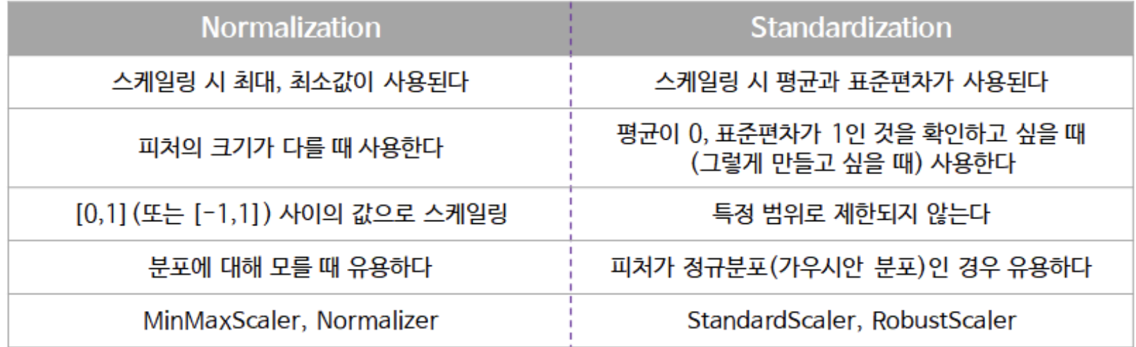
4. 정리
- 데이터 가공 및 변환(전처리)
- 데이터 클렌징
- 인코딩
- 스케일링, 정규화
- 데이터세트 분리
- 교차검층 수행
- KFold
- kfold = KFold(estimator,
- StratifiedKFold
- cross_val_score
cross_val_score(estimator, X_data, y_label, cv=n )- 최적의 하이퍼 파라미터를 위해 GridSearchCV
- 학습
- 예측
- 평가
'💻 파이썬 머신러닝 완벽 가이드' 카테고리의 다른 글
| 파이썬 머신러닝 완벽 가이드 - 5. Classification(2) (앙상블) (0) | 2022.09.29 |
|---|---|
| 파이썬 머신러닝 완벽 가이드 - 5. Classification(1) (결정트리) (0) | 2022.09.29 |
| 파이썬 머신러닝 완벽 가이드 - 4. Evaluation (0) | 2022.09.28 |
| 파이썬 머신러닝 완벽 가이드 - 2. Pandas (2) | 2022.09.26 |
| 파이썬 머신러닝 완벽 가이드 - 1. Numpy (0) | 2022.09.26 |